This article is part of the series dedicated to the most relevant Natural Language Processing tasks. Learn more also the others starting from first article.

Also for an introduction on the basic aspects of Machine Learning read the article Machine learning and applications for industry.

Text Classification

This article discusses the task of text classification.

With text classification we refer, in fact, to the use of supervised approaches of classification type, with the goal of associating textual content with characteristics and classes defined a priori.
Examples of text classification are:

• Sentiment Analysis: for example classify reviews with respect to sentiment (negative and positive)
• Ticket Classification: associate support tickets to the reference category, rather than by urgency
• Document Tagging: classify textual content by associating them with multiple textual classes

These are just some of the possible applications that can be achieved through text classification. Fall within this fiel, all applications that consist in classifying textual contents with respect to a set of labels or classes defined a priori.

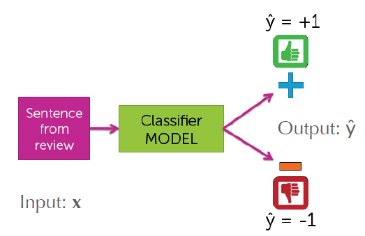
In relation to the examples listed, we can collect the textual classification tasks with respect to three different types:

• Binary classification: the number of classes/labels to associate the contents with is equal to two
• Multiclass classification: the number of classes/labels to associate the contents with is equal to n, with n> 2
• Multiclass multilabel classification: multiclass classification where each content can be associated with more than one class, and therefore have more than one label

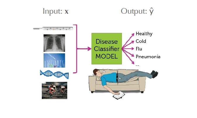
To face a textual classification task according to one of these approaches it is necessary to carry out these three steps:

• label the data: build a training set of textual contents labeled with the features against which you want to perform the classification
• transform and process the text: the textual contents need both a preprocessing phase, necessary to put the textual content into a more suitable form for the task to be carried out, and a phase of transformation of the contents to make them readable and analysable by the algorithms of machine learning that can be used
• model training: the actual phase of training the model using some reference algorithm

Let's see in the following sections how to accomplish this.

Data labeling

The data labeling phase is fundamental to be able to train a Machine Learning model for text classification. Being a supervised approach, nothing can be done without labeled data.

It may happen that you want to build applications for which you already have labeled data. This is because you already have a historian of data tagged thanks to the work done in the past by users, rather than by the employees of the task.
Let's think about the Ticket Classification task.
If the goal is to create a Machine Learning model capable of classifying support tickets with respect to their category, i must have a dataset of past tickets tagged with their respective categories.
I could easily find this data by using all the past tickets that employees have already associated with their categories when they did this work "by hand" to direct the ticket to the most suitable department or person. In a context of this type, it is enough for me to find the data and place them in a readable and usable form for training. Typically a csv file.

If you do not have labeled data available, and therefore only have the textual content to be used for training, then you can use textual annotators to tag the data in an agile and efficient way.
Doccano, for example, is a well structured and open source annotator.
Another annotator, this one for a fee, is Prodigy. It is an advanced and enhanced annotator through the concept of active learning; is developed by Explosion.ai, creators of the opensource library of NLP Spacy.

Once annotated, the data can be easily exported in csv format and then read and manipulated through ad hoc libraries such as Pandas.

Preprocessing and data transformation

1. Preprocessing and cleaning of the text

L'attività di trasformazione e preprocessing dei dati è molto importante in qualsiasi task di Machine Learning, ma nel contesto della Classicazione testuale e più in generale dell'elaborazione del linguaggio naturale è molto rilevante.

Textual content generally contains a lot of information within it, and not all of this information is relevant to the Classification to carry out.
Much of the textual content very often has no relevance to the result produced; on some occasions it can represent instead noise that distorts the classification produced by the model.
For example in the context of Sentiment Analysis, in a review, I can find adjectives like very good rather than very bad which have a specific weight in identifying the sentiment of the content. Other terms, on the other hand, say nothing in this sense.

Furthermore, in natural language a concept can be expressed with terms that have the same root but different declension. Those terms represent the same concept, but having a different declination the Machine Learning model could make it difficult to understand it. And punctuation, too, very often just introduces noise into the text analysis.

For all these reasons it is very important to carry out preprocessing activities of the text in order to minimize all effects as much as possible unwanted caused by irrelevant information present in the text.

These activities can be of different types and deeply linked to the task that is taking place. However, there are some preprocessing activities that they are almost always done when approaching nlp tasks.

A very simple first activity is that of tokenization of the text.
The following actions can then be performed:

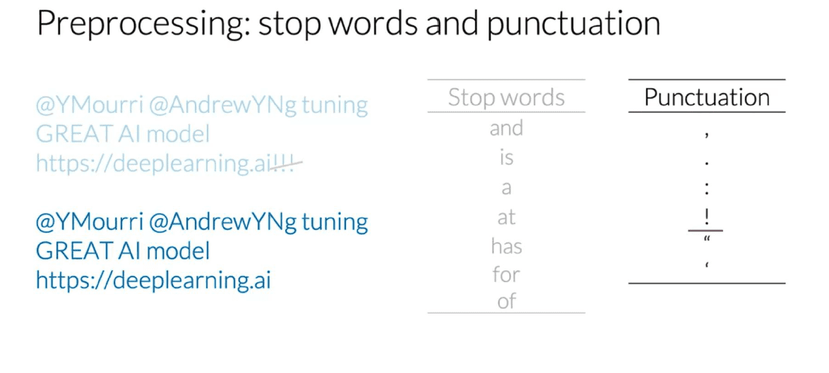
• Remove stopwords: remove from the text all those parts of the speech which in a language do not usually represent information relevant, such as articles, propositions, conjunctions, etc... Furthermore, this activity can be carried out by stopping on the basis of a your own list of words to remove, based on the context and the type of domain you are working on.
• Remove punctuation: punctuation almost never represents relevant information and therefore better to remove it

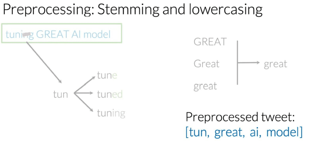
• Stemming: stemming is a very common process in search engines which consists in reducing a term from the inflected form to its root, with the aim of minimizing the effect of the presence of different morphological variations which however have the same semantic meaning. There are two approaches to stemming. A first based on a dictionary, similar to what happens for the removal of stopwords. A second rule-based algorithmic type, for example Porter's Stemmer.
• Lowercasing: transform all text into lowercase characters in order to avoid differentiation based on the character

NLP libraries like Nltk or Spacy offer pre-defined functionality to perform these tasks.
Let's see for example how to carry out these activities through Nltk.

from nltk.corpus import stopwords  
from nltk.tokenize import word_tokenize
from nltk.stem import PorterStemmer 
  
example_sent = """This is a sample sentence, 
                  showing off the stop words filtration."""

# stopwords list 
stop_words = set(stopwords.words('english'))

# stemmer
ps = PorterStemmer() 

# tokenization
word_tokens = word_tokenize(example_sent)  

# stoppping
filtered_sentence = [w for w in word_tokens if not w in stop_words]  

# stemming
stemmed_sentence = [ps.stem(w) for w in filtered_sentence]
  
print(word_tokens)  
print(filtered_sentence)
print(stemmed_sentence)   

2. Text transformation

Once the preprocessing activities on the text have been completed, an important step follows which is the transformation of the contents into a form such that it can be given as input to the Machine Learning algorithms.
Algorithms are not able to directly analyze textual words, and therefore a transformation activity must be carried out in a representation numerical and/or vectorial.

There are several methods for representing textual content. Each of this representation uses the concept of vocabulary. Let's see what they are and how they work.

Bag of Words

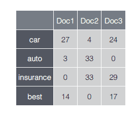
The Bag of Words model consists of a vector representation where each textual content is transformed into a V-dimensional vector, with V representing the cardinality of the vocabulary. In particular we will have that each component of the vector will assume a value equal to zero if the term is not present, otherwise a corresponding value the number of occurrences of that term in the text.

Tf-idf

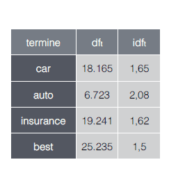
Tf-Idf stands for Term Frequency/Inverted Document Frequency. It is a vector representation similar to that of the Bag of Words method, but for the terms present in the text, rather than the number of occurrences, this value Tf-Idf is used, defined as the ratio between the Term Frequency and the Inverse Document Frequency. The Term Frequency is the frequency of the term within the document. The Inverse Document Frequency is a measure of how much the term occurs within the entire corpus (in how many documents essentially). Compared to the Bag of Words model, this representation therefore emphasizes "relevant" terms such as those that:

• appear frequently in a document ("common locally")
• appear frequently in the corpus ("rare globally") Given these characteristics, this representation is therefore always preferred to the Bag of Words one, which is simpler and therefore less full of meaning.

Text to sequence of numbers

A final representation, mainly used in the context of neural networks, is that which involves transforming each textual content into one sequence of integers, where each integer maps a specific token into a specific vocabulary. This representation is very often used together with the use of Word Embedding.

The chosen representation, very often, depends on the algorithm used and the type of task to be faced. In the vast majority of cases the approach is to use a Tf-Idf model with "classic" algorithms, and a Text to Sequence representation with Deep Learning approaches. In the next section we will see the application and use of these transformations, in the context of the actual training of models for textual classification.

Model training

We have seen what are the best practices regarding text processing and transformation. Now let's see how to train our models. Various algorithms are present at the state of the art which, depending on the context, prove to be very suitable for the classification task textual. Among the classic approaches we find Bayesian Classifier, Support Vector Machine, Logistic Regression. On the other hand, among the approaches of Deep Learning types, convolutional networks are very effective, but in some cases also recurring networks.

Here are two examples of model training that can rank support tickers against their category. using first a Bayesian Classifier and then a Convolutive Neural Network.

The integral code for these examples and also for other examples with others among the algorithms mentioned, are present on the repository Github related to this series of articles. In the repository you will find the source code of the examples described and executable in well documented jupyter notebooks.

1. Textual classification with Bayesian Classifier

In our case we will use a Bayesian Classifier in the so-called "naive" version (Naïve Bayes Classifier). It is a simplified Bayesian Classifier with an underlying probability model making the hypothesis of independence of characteristics, i.e. it assumes that the presence or absence of a particular attribute in a textual document is unrelated to the presence or absence of other attributes

To train the model we will use the Scikit-Learn library.

Let's assume that we have our tickets already preprocessed through the techniques already seen in the previous sections in a csv file. Moreover for each textual content we know the category expressed through a numerical identifier.

The first step we must take is to read the data and create the training set for the training on the one hand, on the other the test set for validation.

To do this we first import the contents of the csv into a Pandas dataframe. We then extract the text and labels and build two special lists.

import pandas as pd

df_tickets = pd.read_csv('input/all_tickets.csv')


text_list = df_tickets['body'].tolist()
labels_list = df_tickets['category'].tolist()

Now we are going to transform the list of textual contents into a representation of the Tf-Idf type. To do this we use functions defined by the library. Once that's done, let's split the whole thing together into training and test sets.

from sklearn.feature_extraction.text import CountVectorizer
from sklearn.feature_extraction.text import TfidfTransformer
from sklearn.model_selection import train_test_split

X_train, X_test, y_train, y_test = train_test_split(text_list, labels_list, test_size=0.1, random_state=0)

count_vect = CountVectorizer()
vectorized_data = count_vect.fit_transform(X_train)

tfidf = TfidfTransformer()
X_train = tfidf.fit_transform(vectorized_data)

At this point we move on to the actual training and then to the evaluation of the performances obtained by calculating through predefined functions the accuracy achieved and the confusion matrix relating to the test set.

from sklearn.naive_bayes import MultinomialNB
from sklearn.metrics import f1_score, accuracy_score, classification_report

mnb = MultinomialNB()
mnb.fit(X_train, y_train)

pred = mnb.predict(X_test_tfidf)

#print(f1_score(y_test, pred))
print(accuracy_score(y_test, pred))
#print(precision_score(y_test, pred))
confusion_matrix(y_test, pred)

The model at this point can be saved in pickle format and then used for your own purposes. The model takes in I input a Tf-Idf representation and not the natural text, so before giving the textual input content to the model, it must always be converted into the chosen representation (in this case Tf-Idf).

Scikit-learn provides a tool that simplifies these aspects and actually allows you to define an end-to-end model, i.e. a model that takes the text directly as input and outputs the desired classification. This happens through the class sklearn.pipeline.Pipeline, through which it is possible to define in a single object the list of all the transformations and actions to be performed. The previous code will be partially replicated by the following code.

from sklearn.feature_extraction.text import CountVectorizer, TfidfTransformer
from sklearn.naive_bayes import MultinomialNB
from sklearn.pipeline import Pipeline

text_clf = Pipeline([
        ('vect', count_vect),
        ('tfidf', TfidfTransformer()),
        ('clf', MultinomialNB())
    ])

Another very useful function to mention, defined by the class sklearn.model_selection.GridSearchCV, is the Grid Search to perform parameter optimization quickly and easily.

Both the concept of Pipeline and Grid Search are explored and used in the code present on the Github repository.

2. Textual classification with convolutional neural networks

Another algorithm very suitable for carrying out textual classification tasks is that of convolutional neural networks, in particular networks with 1-dimensional convolutional layers, which carry out temporal convolution operations, while the 2-dimensional convolutional layers adapt more to image processing and analysis. For further information on the differences: https://missinglink.ai/guides/keras/keras-conv1d-working-1d-convolutional-neural-networks-keras/.

Now let's see how to train a model for the classification of tickets through algorithms of this type. We do this using Tensorflow Keras as a support library. We always assume that our pre-processed and "cleaned" tickets are available in a csv file.

Comer for the approach with the Bayesian Classifier, first we import the contents of the csv in a Pandas dataframe. We then extract the text and labels and build two special lists.

import pandas as pd

df_tickets = pd.read_csv('input/all_tickets.csv')


text_list = df_tickets['body'].tolist()
labels_list = df_tickets['category'].tolist()

Now let's move on to the data transformation activity, and in this case we use a transformation of type text to sequence of numbers. Every textual content is transformed into a sequence of integers, where each whole map a term in a dedicated vocabulary. To do this we use a utility defined by Keras with the class tf.keras.preprocessing.text.Tokenizer. Once the data has been transformed, the split into train and test set is done and then the sequences are padded to a maximum length defined by analyzing the dataset a priori. Labels are also transformed through a LabelEncoder, although for this dataset the labels are already defined as integers. This step it is essential when the labels are not integers.

from tensorflow.keras.preprocessing.text import Tokenizer

tokenizer = Tokenizer(split=' ')
tokenizer.fit_on_texts(text_list)
X = tokenizer.texts_to_sequences(text_list)

values = np.array(text_list)
# integer encode
label_encoder = LabelEncoder()
label_encoder.fit(values)
Y = label_encoder.transform(text_list)

X_train, X_test, Y_train, Y_test = train_test_split(X, Y, test_size=0.1, random_state=42)

# padding sequences to maxlen
print('Pad sequences (samples x time)')
X_train = sequence.pad_sequences(X_train, maxlen=maxlen)
X_test = sequence.pad_sequences(X_test, maxlen=maxlen)
print('x_train shape:', X_train.shape)
print('x_test shape:', X_test.shape)

At this point follows the definition of the model architecture, the definition of the hyperparameters and the actual training. Training is controlled by an Early Stopping approach to prevent any Overfitting phenomena.

from tensorflow.keras.models import Sequential
from tensorflow.keras.layers import Dense, Dropout, Activation
from tensorflow.keras.layers import Embedding
from tensorflow.keras.layers import GlobalAveragePooling1D, Conv1D, GlobalMaxPooling1D
from tensorflow.keras.callbacks import EarlyStopping

batch_size = 32 # batch size
epochs = 100 # number of epochs
filters = 100
kernel_size = 1
hidden_dims = 100
embedding_dim = 100

print('Build model...')
model = Sequential()

# we start off with an efficient embedding layer which maps
# our vocab indices into embedding_dims dimensions
if use_pretrained_embeddings: 
    model.add(Embedding(max_features+1,
                        embedding_dim,
                        input_length=maxlen
                        , weights = [embedding_matrix], trainable = True))
    print("using pretrained embeddings")
else:
    model.add(Embedding(max_features+1,
                        embedding_dim,
                        input_length=maxlen))
    print("using embeddings from scratch")
model.add(Dropout(0.2))

# we add a Convolution1D, which will learn filters
# word group filters of size filter_length:
model.add(Conv1D(filters,
                 kernel_size,
                 padding='valid',
                 activation='relu',
                 strides=1))

# we use max pooling:
model.add(GlobalMaxPooling1D())

# We add a vanilla hidden layer:
model.add(Dense(hidden_dims))
model.add(Dropout(0.2))
model.add(Activation('relu'))

# We project onto a single unit output layer, and squash it with a softmax:
model.add(Dense(n_outputs))
model.add(Activation('softmax'))

model.compile(loss='sparse_categorical_crossentropy',
              optimizer='adam',
              metrics=['accuracy'])

callback = EarlyStopping(monitor='val_loss', min_delta=0, patience=5, verbose=0, mode='auto',
    baseline=None, restore_best_weights=False)

history = model.fit(np.array(X_train), np.array(Y_train),
              batch_size=batch_size,
              epochs=epochs,
            validation_split=0.1, callbacks = [callback])

The model can also be saved in this case and reused where necessary. And just as with Scikit Learn it is possible implement an end-to-end approach to avoid having to carry out transformations on the input every time. One possible strategy is present on the documentation by Tensorflow Keras.

For further information see the associated notebook on the Github repository.

3. Evaluations and comparisons

Which of the two approaches is the best? Which achieves the best level of accuracy?

There are several metrics and evaluation approaches that can be used to clarify this. In the case of textual classification, and more generally in the classification approaches, Accuracy, Precision, Recall, F1-score are fundamental metrics to calculate and analyze. Another always very useful tool is the confusion matrix, which allows you to visualize false positives and negatives.

Let's see the results of the training through the classification reports produced in the evaluation phase. These reports show precision, recall, accuracy, and other metrics in a single table, with focus on both classes and overall performance.

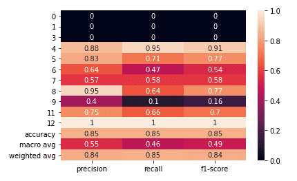
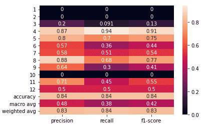
For this task the two classifiers have very similar performances as we can see. Preform the slightly better Bayesian classifier. But it's not always like this.

Convolutional neural networks, for example, prove to be very powerful when the classification depends on very identifying features. To example let's imagine we want to classify business documents with respect to the customer. Information such as the customer's name rather than VAT number they are very useful information to understand which customer the document refers to. In cases like these, neural networks achieve results of very high accuracy.
The Bayesian Classifiers, on the other hand, prove to be very accurate in the vast majority of cases. Even if they don't always reach the levels of accuracy of convolutional neural networks, their strength is to return very significant confidence values ​​associated with the classification, and with well-defined thresholds. This happens because the Bayesian Classifier is a probabilistic model.

Neural networks also return a confidence value associated with the classification, which, however, cannot be considered entirely a value probabilistic, as it is the highlight of the application of a Softmax to the output layer of the network. So in fact it should be considered as a transposition in the space of probabilities of the result produced by the network. For these reasons, the confidence value must be interpreted differently and not always manages to express the desired differences.

Conclusions

Summarizing the textual classification allows us to catalog our textual contents with respect to characteristics of different types. The ability to group textual content in an automatic and intelligent way can represent a considerable added value for a company for example. Think of a management software that allows the filing of corporate documents of various kinds in separate spaces; through an instrument text classification based on Machine Learning, you can automatically catalog the document in correct space, based on customer rather than type. Another example can be a support system for CSS. Similarly to what has been done in the examples seen, they can be classified automatically incoming tickets based on category or urgency to help in the task of assigning tickets to the relevant departments.

So what are you waiting for? Take advantage of the potential offered by Machine Learning to automatically classify and extract information from the text in order to make your application smarter. Have fun with the notebooks on the Github repository to test the algorithms seen in the examples and also other algorithms such as Support Vector Machines or LSTM networks.
Then reuse these algorithms to build your own text classification models to use in support of your application.

In this article, only some of the most relevant topics regarding textual classification have been cited. Kamran Kowsari studied all the aspects related to this task through a very complete paper, explaining in an excellent way advantages and disadvantages. This is a treatment that touches on many aspects that concern not only the task of textual classification, but in general the whole world of Natural Language Processing. If you are into NLP you can't miss it.

Referenced Paper: Kowsari, K., Meimandi, K. J., Heidarysafa, M., Mendu, S., Barnes, L. E., & Brown, D. E. (2019). Text Classification Algorithms: A Survey.

Medium Article: Text Classification Algorithms: A Survey.